The big macroeconomic question of drivers of current
inflation also found its way into formal empirical analyses. The starting shot
of this discussion (probably) dates to Adam’s
Shapiro paper using VAR methodology, which was later replicated
for euro zone by ECB authors. Similarly, Ricardo Trezzi and co-authors have new
paper using similar VAR methodology.[1]
Mostly, these papers lead to conclusion that both supply and
demand are driving inflation, and roughly to a similar degree. For example,
here is picture for euro zone from the ECB authors (all other pictures also are for euro zone):

However, looking at considering the picture from previous
posts,
what these papers are really saying is that the most recent shock has been a
demand shock, as we observe both increase in prices and quantities. This is the
example of airline tickets, as in 2022 we observed increase in prices and
quantities. So, using the terminology of “driving” vs. “causing”, these estimates
are estimates of what is driving the inflation, rather that what is causing
it.
However, even accepting this, there are reasons why these
estimates might be imperfect. This has to do with several problems with their
identification strategy, which while being neat and probably the best we can
do, is still far from perfect for the messy reality. Therefore, I personally
think of these estimates as good starting point, but one that probably provides
an upper bound on demand-driven component of inflation. Below is discussion of
several reasons why.
Identification of forecast errors
All the papers proceed along similar way. They first
estimate VAR model, which links price and quantity developments to previous
price and quantity developments in the typical autoregressive fashion. For each
period they then decompose the actual movement in the prices and quantities
into movements that are “expected”, that is predicted by the model in absence
of the shocks, and movements that are caused by shocks, i.e. not predicted by
the model. The difference between those are the forecast errors, and these
forecast errors then form the basis of the identification strategy: a
combination of positive forecast errors for quantity and prices suggests demand
shocks, while negative forecast error for quantity and positive for price
suggests supply shocks.
However, this identification strategy crucially depends on
identification of forecast errors. And the identification of what is “forecast
error” of course depends on what is “expected”. And therein lies the problem.
While autoregressive process is a reasonable description of evolution of
macroeconomic variables before the pandemic, it is pretty woeful description of
developments during pandemic. Why? Because during pandemic shocks are reversed
rather than propagated.
For example, if you end up with another wave of pandemic in
fall of 2021, this means a decrease in quantity of flights, which is however
expected to be reversed pretty soon. In other words, a negative movement is
followed by positive movement. In contrast, VAR model will expect that that negative
movement will be followed by further negative movements. While this is entirely
plausible description of usual developments, we are not in the realm of usual.
In other words, the model is estimated on data coming from different
data-generating process than the recent observations.
A nice example of this comes the paper by Ricardo Trezzi an
co-authors. Consider the period from July 2020 onwards. According to their model
there was a large positive forecast error for output (proxied by industrial production),
meaning that output was higher than the VAR model predicted.

But is this reasonable? In other words, was it reasonable to
expect output to remain at July 202 levels throughout the 12 months after July
2020? I don’t think so – there was general expectations for economic output to
increase following the drop and initial rebound during pandemic. In other
words, from non-model perspective, there wasn’t a surprise increase in
output, and hence there wasn’t a positive forecast error for output. Of course,
if we were to change the forecast errors for the model variables, then we would
also end up with completely different set of structural shocks, which we are
after.
The point is that the VAR models are going to systematically
consider post-pandemic rebound as positive forecast errors in terms of
quantity. And since this rebound naturally coincides with increases in prices, then we will conclude
that these are positive demand shocks, and hence label resulting increase in
prices as “demand driven”. Of course, insofar as these increases in quantity
are not real surprise – most forecasters expected these increases in output as
part as post-pandemic rebound, so they are only surprise in the context of our
VAR model – we are misidentifying forecast errors and hence misidentifying the
shocks.
The ECB authors actually point towards this problem in the
conclusion to their piece, highlighting the same issues I discussed in detail
here:
In addition, developments
in quantities and prices have clearly been exceptional since the start of
the pandemic and have been influenced by many special factors, making it more difficult
to build a reliable model as a basis for classification based on the
signs of its errors.
This is exactly the crux of the matter: to identify
structural shocks based on sign restrictions, you need to identify forecast
errors for your variables. And for that you need a model which will do this
reliably during the pandemic period, which is bit too much to expect from model
estimated on pre-pandemic data. In other words, I would not be raising this
issue if we were talking about overall pre-pandemic period, where I do buy that
VAR model can identify shocks; pandemic period is different metter.
Identification via sign restrictions and issue of timing
Related problem of the identification strategy is the
problem of timing of shocks and effects and their relationship to sign
restrictions. The idea behind the identification strategy is that when demand
or supply shock happens, it affects prices immediately. This corresponds to the
micro-economic concept of equilibrium. And while this is reasonable assumption
for some markets, it is not for other markets, simple because there are
sometimes delays in reaction in prices. This can be because prices are set by
firms, and such price settings is updated only once in a while. Or it can be
simply because price discovery takes time.
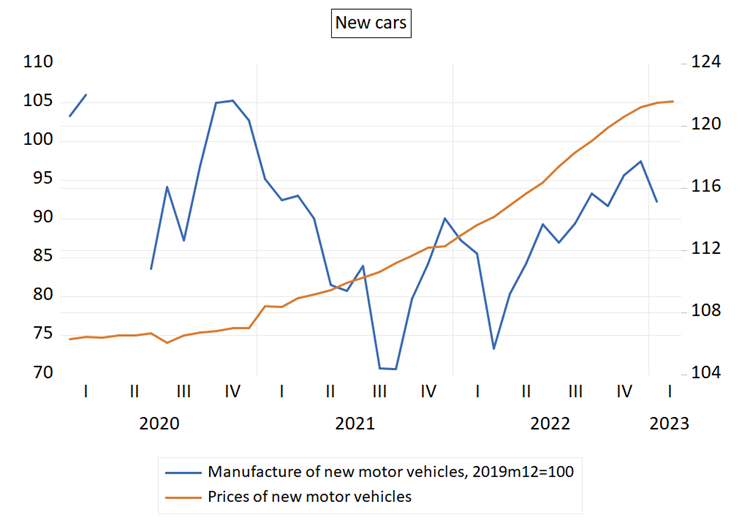
For the former, consider new car prices in euro zone. We
know that car production has collapsed in 2021 due to chip shortage (see picture
below). This is unambiguously a negative supply shock, which in standard
microeconomics should mean higher prices in 2021. However, looking at
the time series plot of new car prices you would conclude there was major shock
in 2022, not in 2021. (Of course, there
was additional shock coinciding with the invasion, but that was quickly
reversed).
Why is this a problem? It is problem because of the
concurrent evolution of output. New car production has rebounded throughout
2022, as the supply chain problems gradually unwound. From perspective of our
VAR model this is going to be unexpected increase in quantity. And this
unexpected increase in quantity coincides with unexpected increase in price.
Therefore, our model will assign this increase in price to a demand shock,
consistent with the identification strategy based on sign restrictions. But we
know that the increase in prices is not due to demand shock, or at least not to
any significant degree. Instead, it is a delayed price effect of previous
supply shock. This is then example how the identification strategy fails in
presence of delayed price effects due to price adjustment being a gradual
process in situation when firms set prices.
Meanwhile, used car prices are best described as determined
by price discovery, rather that set by firms, and hence provide example of slow
price discovery. Used car prices in euro zone follow similar profile as new car
prices, only more extreme: there is no price increase in first half of 2021, and
significant increase comes only from 2022 onwards.[2]
Again, this is a result of supply chain problems affecting car production
throughout 2021, which showed up in price data only in 2022. But insofar as
2022 is time when quantity of used cars traded increases, corresponding to
increases in new car production, we will again observe higher quantity and
prices together, and assign this to demand shock.

These are just two examples of these kind of issues, illustrating
a broader point: our identification strategy based on sign restrictions is
going to fail if the changes in prices are delayed relative to the shocks
affecting output.
Multiple shocks
Another related issue is the issue originating in multiple
shocks. In principle, the example discussed in my previous
post was a somewhat philosophical example of possible problems caused by
multiple shocks. But this problem can arise even in more prosaic situations.
The source of the problem is that the identification
strategy relies on the overall change in quantities, but this can be misleading
if supply and demand shocks happen together and push in opposite direction.
Most naturally, in the post-pandemic, post-invasion period we are likely to get
negative supply shocks and positive demand shock. This is problem for two
reasons.
First, we will end up assigning the whole price effect to
either demand or supply shock, even though it is due to both. Second, the
overall quantity effect does not need to indicate which shock was “bigger”, as
the quantity effect also depends on the relative elasticities. Picture below
shows a large negative supply shock and small demand shock which nevertheless
result into higher quantity.

Most importantly, these two problems interact together. In
the above example looking at prices and quantities we assign things to demand
shock, as quantity and price increased. And we will assign the whole price
change to demand shock.
As an example, consider restaurant prices. In the aftermath
of the Russian invasion of Ukraine the supply has decreased dramatically in
that restaurants were willing to supply only at much higher prices as their
costs have surged. At the same time, demand has likely increased due to the
post-pandemic re-opening. If we are willing to assume that demand at this point
in time was inelastic – people were eager to go to restaurants after 2 year
hiatus, then we could easily assign the complete increase in prices to demand
shock, even though most of it was due to supply shock.
This is made worse by the delayed price effects. Presumably,
pandemic itself meant negative supply shock in so far as many restaurants did
not survive the lockdowns. But this was likely not reflected in prices during
the pandemic, when restaurants fighting for survival were unlikely to increase
prices. This price increase came only when the re-opening happened. And at that
point we observe increase in quantities and prices and conclude we are seeing
positive demand shock. In reality, increase in prices was at least partly, if
not dominantly down to earlier negative supply shock.
The general point is that in presence of multiple shocks
going in opposite directions, sign restrictions might lead to misleading identification.
Again, to their credit, the ECB authors point out this problem in their
conclusion:
Second, the disaggregated approach cannot quantify how large the supply and demand contributions are for each component. This could introduce a bias if, for example, the role of supply factors for components classified as predominantly demand-driven is on average much larger than the role of demand factors for components classified as predominantly supply-driven.
In other words, in presence of multiple shocks, the identification based on sign restrictions becomes potentially problematic.
Conclusion
Overall, while the identification approach based on sign
restrictions in VAR models are clever and definitively a step in the right
direction - especially those based on detailed data - I think that people should
not be putting so much weight on the resulting estimates. I would be willing to
put a lot of weight on them during normal periods where we are not dealing with
multiple major and unprecedent shocks. However, in current environment where there
are likely multiple shocks, that are both large and unprecedented, I think that
the estimates need to be taken with large grain of salt. And this is not only because
potential noisiness of the estimates, but also because I think that with large probability
the estimates are also biased: note that the problems will typically lead to
higher estimate for demand component, rather than higher estimate of supply
component.
And then there is also the related issue of interpreting
these results, something that I touched upon in previous
post. Even if we accept the estimates of demand driven component at face value,
these estimates do not say what some people claim they do. Specifically, they don’t
say that aggregate demand is running abnormally hot; at most, they might imply
that aggregate demand is has (a) recovered strongly after the pandemic shock,
(b) has recovered to larger degree than aggregate supply.
[1] While
there are other papers using different approaches, I will focus only on the
papers using VAR methodology here.
[2] At
least as far as CPI data can be trusted – anecdotal evidence would suggest that
prices started rising significantly already in 2021, same as in US. But of
course, given its nature, it is hard to know how much should we trust anecdotal
evidence.
No comments:
Post a Comment